%matplotlib inline
import matplotlib
import seaborn as sns
sns.set()
matplotlib.rcParams['savefig.dpi'] = 144
import numpy as np
import pandas as pd
import matplotlib.pyplot as plt
¶ Linear Regression and Machine Learning
The power of quantitative sciences comes from the insight we can derive from mathematical relationships between different measurements. We can use these insights to make predictions about what will happen in the future. The simplest possible relationship between two variables is a linear relationship
If we can measure some pairs, we could calculate our model parameters and . Then we could predict in the future based on , or even try to influence in the future by controlling .
gas = pd.read_csv('./data/gas_consumption.csv', names=['tax', 'income', 'highway', 'drivers', 'gas'])
gas.head()
| tax | income | highway | drivers | gas | |
|---|---|---|---|---|---|
| 1 | 9.0 | 3571 | 1976 | 0.525 | 541 |
| 2 | 9.0 | 4092 | 1250 | 0.572 | 524 |
| 3 | 9.0 | 3865 | 1586 | 0.580 | 561 |
| 4 | 7.5 | 4870 | 2351 | 0.529 | 414 |
| 5 | 8.0 | 4399 | 431 | 0.544 | 410 |
gas.shape
(48, 5)
from ipywidgets import interact
def plotter (feature):
    plt.plot(gas[feature], gas.gas, '.',c='b')
    plt.xlabel(feature)
    plt.ylabel('Gas consumption (millions of gallons)')
menu = gas.columns
interact(plotter, feature=menu);
interactive(children=(Dropdown(description='feature', options=('tax', 'income', 'highway', 'drivers', 'gas'), …
¶ Simple Regression (one feature)
let's use one of the features. lets see how the value we want to predict, the gas consumption, varies with the percentage of population of these drivers.
gas.plot(x='drivers', y='gas', kind='scatter', c='b')
plt.xlabel('% of population driving')
plt.ylabel('Gas consumption (millions of gallons)');
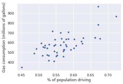
We could try to draw a line describing the trend in the data, but which is the best one?
gas.plot(x='drivers', y='gas', kind='scatter', c='b')
plt.xlabel('% of population driving')
plt.ylabel('Gas consumption (millions gallons)')

plt.plot([.4, .8], [300, 1000], c='r')
plt.plot([.4, .8], [200, 1100], c='g');
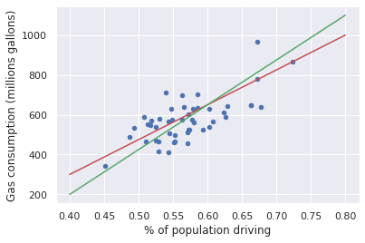
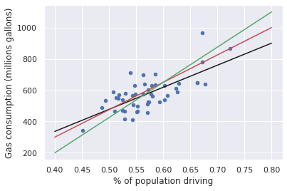
In order to compare the different trend lines we need to define a metric for how well they describe the actual data. The metric should reflect what we value about our trend line. We want our trend line to reliably predict a y-value given an x-value, so it would be reasonable to construct our metric based on the error between the trend line and the y-values.
We want to make the total error as small as possible. Since sometimes the errors will be positive and some will be negative, if we add them together they might cancel out. We don't care if the error is positive or negative, we want the absolute value to be small. Instead of minimizing the total error, we'll minimize the total squared error. Often we divide it by the number of data points, , which is called the mean squared error (MSE).
Since depends on our model parameters and , we can tweak our model (the trend line) until the MSE is minimized. In the language of machine learning, the MSE would be called the cost function or loss function.
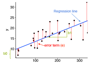
In the above diagram,
- x is our dependent variable which is plotted on the x-axis and y is the dependent variable which is plotted on the y-axis.
- Black dots are the data points i.e the actual values.
- bo is the intercept which is 10 and b1 is the slope of the x variable.
- The blue line is the best fit line predicted by the model i.e the predicted values lie on the blue line.
The vertical distance between the data point and the regression line is known as error or residual. Each data point has one residual and the sum of all the differences is known as the Sum of Residuals/Errors.
from sklearn.linear_model import LinearRegression
linreg = LinearRegression(fit_intercept=True)
linreg.fit(gas[['drivers']], gas['gas'])

gas.plot(x='drivers', y='gas', kind='scatter', c='b')
plt.xlabel('% of population driving')
plt.ylabel('Gas consumption (millions gallons)')

x = np.linspace(.4, .8).reshape(-1, 1)
print(x.shape)
predictions = linreg.predict(x)
print(linreg.score(gas[['drivers']], gas['gas']))
plt.plot(x, predictions, c='k')
plt.plot([.4, .8], [300, 1000], c='r')
plt.plot([.4, .8], [200, 1100], c='g');
(50, 1)
0.4885526602607474


/home/sulaiman/anaconda3/lib/python3.9/site-packages/sklearn/base.py:450: UserWarning: X does not have valid feature names, but LinearRegression was fitted with feature names
  warnings.warn(
predictions.shape
(50,)
np.linspace?
(linreg.intercept_, linreg.coef_[0])
(-227.3091174945256, 1409.8421113288002)
¶ Gradient descent
How did we find the model parameters that minimize the cost function? Let's plot the cost function with respect to to get an idea.
beta0 = linreg.intercept_
beta1 = np.linspace(1300, 1500)

MSE = [((gas['gas'] - (beta0 + m * gas['drivers']))**2).sum() for m in beta1]

plt.plot(beta1, MSE)
plt.xlabel('Beta1')
plt.ylabel('MSE')
Text(0, 0.5, 'MSE')
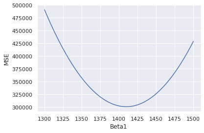
If we started with some initial guess , we could simply follow the slope of the MSE downhill with respect to . We could calculate the MSE around 1300 to work out which way is downhill, and then update in that direction. With each step we move closer and closer to the bottom of the valley at 1409.
This method of always going downhill from where we are is called gradient descent. In general the loss function could be very complicated and we won't be able to solve where the minimum is directly. Gradient descent gives us an algorithm for finding our way to the minimum when we don't know where it is in advance.
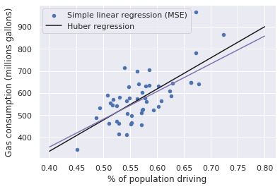
For example, the HuberRegressor also optimizes a linear model, but uses a more complicated loss function. The Huber loss is less influenced by outliers than the MSE.
from sklearn.linear_model import HuberRegressor
huber = HuberRegressor(fit_intercept=True, alpha=0)
huber.fit(gas[['drivers']], gas['gas'])
gas.plot(x='drivers', y='gas', kind='scatter', c='b')
plt.xlabel('% of population driving')
plt.ylabel('Gas consumption (millions gallons)')

x = np.linspace(.4, .8).reshape(-1, 1)
plt.plot(x, linreg.predict(x), 'k-')
plt.plot(x, huber.predict(x), 'm-')
plt.legend(['Simple linear regression (MSE)', 'Huber regression']);
/home/sulaiman/anaconda3/lib/python3.9/site-packages/sklearn/base.py:450: UserWarning: X does not have valid feature names, but LinearRegression was fitted with feature names
  warnings.warn(
/home/sulaiman/anaconda3/lib/python3.9/site-packages/sklearn/base.py:450: UserWarning: X does not have valid feature names, but HuberRegressor was fitted with feature names
  warnings.warn(
¶ Multivariate regression
Looking again at our DataFrame, we see we have other variables we could use to predict gas consumption.
from ipywidgets import widgets

feature_desc = {'tax': 'Gas tax', 'drivers': '% of population driving', 'income': 'Average income (USD)', 'highway': 'Miles of paved highway'}

def plot_feature(column):
    plt.plot(gas[column], gas['gas'], '.')
    plt.xlabel(feature_desc[column])
    plt.ylabel('Gas consumption (millions gallons)')

dropdown_menu = {value: key for key, value in feature_desc.items()}

widgets.interact(plot_feature, column=dropdown_menu);
interactive(children=(Dropdown(description='column', options={'Gas tax': 'tax', '% of population driving': 'dr…
To use all of these predictors (called features), we will need to fit a slightly more complicated function
or more generally
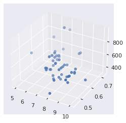
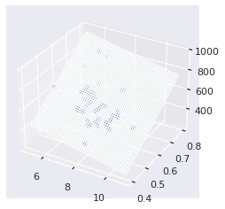
where labels different observations and labels different features. When we have one feature, we solve for a line; when we have two features, we solve for a plane; and so on, even if we can't imagine higher dimensional spaces.
from mpl_toolkits.mplot3d import Axes3D

# plt.figure(figsize=(10,10))
plt3d = plt.figure().gca(projection='3d');
plt3d.scatter(gas['tax'], gas['drivers'], gas['gas']);
/tmp/ipykernel_19632/726554170.py:4: MatplotlibDeprecationWarning: Calling gca() with keyword arguments was deprecated in Matplotlib 3.4. Starting two minor releases later, gca() will take no keyword arguments. The gca() function should only be used to get the current axes, or if no axes exist, create new axes with default keyword arguments. To create a new axes with non-default arguments, use plt.axes() or plt.subplot().
  plt3d = plt.figure().gca(projection='3d');
linreg.fit(gas[['tax', 'drivers', 'income']], gas['gas'])
LinearRegression()In a Jupyter environment, please rerun this cell to show the HTML representation or trust the notebook.
On GitHub, the HTML representation is unable to render, please try loading this page with nbviewer.org.
LinearRegression()
linreg.score(gas[['tax', 'drivers', 'income']], gas['gas'])
0.6748583388195666
plt3d = plt.figure().gca(projection='3d')

xx, yy = np.meshgrid(np.linspace(5, 11), np.linspace(.4, .8))
z = linreg.intercept_ + linreg.coef_[0] * xx + linreg.coef_[1] * yy
plt3d.plot_surface(xx, yy, z, alpha=.1)
plt3d.scatter(gas['tax'], gas['drivers'], gas['gas']);
/tmp/ipykernel_19632/3426350038.py:1: MatplotlibDeprecationWarning: Calling gca() with keyword arguments was deprecated in Matplotlib 3.4. Starting two minor releases later, gca() will take no keyword arguments. The gca() function should only be used to get the current axes, or if no axes exist, create new axes with default keyword arguments. To create a new axes with non-default arguments, use plt.axes() or plt.subplot().
  plt3d = plt.figure().gca(projection='3d')
from ipywidgets import interact

def plot_cross(tax=5):
    x = np.linspace(.4, .8)
    plt.plot(x, linreg.intercept_ + linreg.coef_[0]*tax + linreg.coef_[1]*x)
    alpha = 1 - abs(gas['tax'] - tax) / abs(gas['tax'] - tax).max()
    colors = np.zeros((len(gas), 4))
    colors[:, 3] = alpha
    plt.scatter(gas['drivers'], gas['gas'], color=colors)

interact(plot_cross, tax=(5,11,1));
interactive(children=(IntSlider(value=5, description='tax', max=11, min=5), Output()), _dom_classes=('widget-i…
X = gas[['tax', 'income', 'drivers']]
y = gas['gas']
from sklearn.pipeline import Pipeline
from sklearn.preprocessing import StandardScaler
pipe = Pipeline([('scaler', StandardScaler()), ('regressor', LinearRegression())])
pipe.fit(X,y)
Pipeline(steps=[('scaler', StandardScaler()),
('regressor', LinearRegression())])</pre><b>In a Jupyter environment, please rerun this cell to show the HTML representation or trust the notebook. <br />On GitHub, the HTML representation is unable to render, please try loading this page with nbviewer.org.</b></div><div class="sk-container" hidden><div class="sk-item sk-dashed-wrapped"><div class="sk-label-container"><div class="sk-label sk-toggleable"><input class="sk-toggleable__control sk-hidden--visually" id="sk-estimator-id-9" type="checkbox" ><label for="sk-estimator-id-9" class="sk-toggleable__label sk-toggleable__label-arrow">Pipeline</label><div class="sk-toggleable__content"><pre>Pipeline(steps=[('scaler', StandardScaler()),
('regressor', LinearRegression())])</pre></div></div></div><div class="sk-serial"><div class="sk-item"><div class="sk-estimator sk-toggleable"><input class="sk-toggleable__control sk-hidden--visually" id="sk-estimator-id-10" type="checkbox" ><label for="sk-estimator-id-10" class="sk-toggleable__label sk-toggleable__label-arrow">StandardScaler</label><div class="sk-toggleable__content"><pre>StandardScaler()</pre></div></div></div><div class="sk-item"><div class="sk-estimator sk-toggleable"><input class="sk-toggleable__control sk-hidden--visually" id="sk-estimator-id-11" type="checkbox" ><label for="sk-estimator-id-11" class="sk-toggleable__label sk-toggleable__label-arrow">LinearRegression</label><div class="sk-toggleable__content"><pre>LinearRegression()</pre></div></div></div></div></div></div></div>
pipe.score(X, y)
0.6748583388195667
Copyright © 2022 Marconi Lab. All rights reserved.